How It Works
This page follows one dataset through the program, step by step, with the figures to match. Every example comes from a
real run on the example dataset that ships with the program (examples/sample.csv: 180 rows, 20 subjects, 22 columns).
You can download that file and repeat each step: csvexample-pk_study.csv.
1. From file to masked dataset
data-obfuscator run does six things in a fixed order. Nothing is sent over a network; the program reads your file and
writes a new folder next to it.
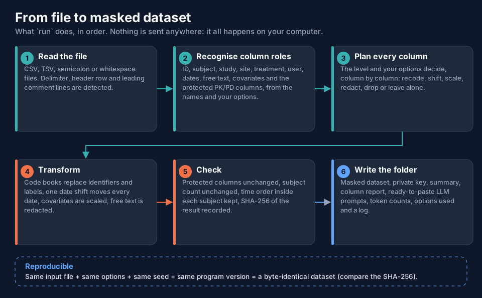
| Step | What happens | Where you see it |
|---|---|---|
| 1. Read | The delimiter (comma, tab, semicolon, whitespace), the header row and any leading comment lines (#, ;, $) are detected. |
[OK] read 180 rows × 22 cols (CSV (comma)) in the terminal |
| 2. Recognise | Each column is given a role from its name (ID, USUBJID, ARM, DATE, WT, ...) unless you named it yourself. |
column_report.txt |
| 3. Plan | The level and your options decide, per column: recode, shift, scale, redact, drop or leave alone. | column_report.txt, config.used.txt |
| 4. Transform | One code book per identifier kind, one date shift for the whole file, one hidden factor per scaled column. | keymap.txt |
| 5. Check | Protected columns unchanged, subject count unchanged, within-subject time order kept. The SHA-256 of the result is recorded. | summary.txt (INTEGRITY) |
| 6. Write | The masked dataset, the private key, the LLM prompts, token counts and a log. | The output folder |
2. How the program sees your columns
The role of a column decides what is done to it. The role comes from the name (the detection table is in the
CONFIGS.md of the project folder); when your names are unusual you tell the program with a role option such as
--site-column (see the Columns and Roles page of the Using the Program section).
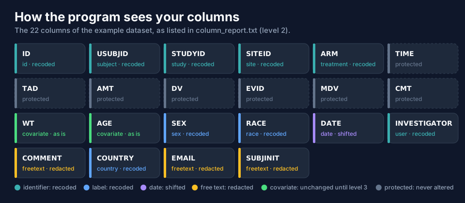
The colours are the whole idea in one picture:
- teal columns identify someone or something (subject, study, site, treatment, user): they are recoded;
- blue columns are labels (sex, race, country): recoded from level 2;
- violet is the date, shifted from level 2;
- amber is free text (
COMMENT,EMAIL,SUBJINIT): redacted from level 2; - green covariates (
WT,AGE): unchanged until level 3, where they are scaled; - grey columns are the PK/PD structure and are never altered.
3. Before and after
Here are the first rows of the example at level 2, next to the original. Only the identifying columns change.
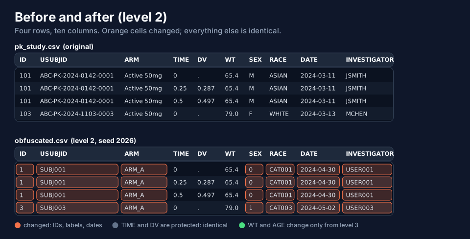
The first record, written out in full:
original : 101,ABC-PK-2024-0142-0001,ABC-PK-2024,0142,Active 50mg,0,0,50,.,1,1,1,65.4,29,M,ASIAN,2024-03-11,JSMITH,.,USA,n.patel.0142@harbor-site.org,RKO
level 2  : 1,SUBJ001,STU001,SITE001,ARM_A,0,0,50,.,1,1,1,65.4,29,0,CAT001,2024-04-30,USER001,.,C001,.,.
TIME, TAD, AMT, DV, EVID, MDV and CMT (0,0,50,.,1,1,1) are byte for byte the same; the weight and the age
(65.4,29) are the same too, because covariates are only scaled from level 3 on.
4. The PK/PD structure survives
Because the PK/PD columns are protected, anything computed from them gives the same answer on the masked data: the concentration–time profile, the dose, the number of observations per subject. The figure shows the same 80 observations before and after masking at level 3.
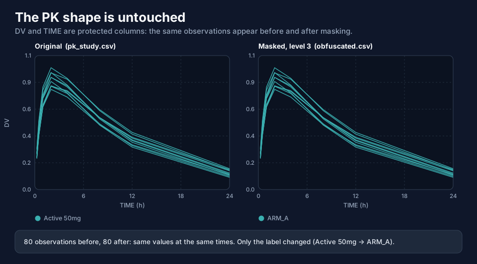
This is what makes a masked dataset worth giving to an LLM: it can fit, plot and explain the data, and the answers are right, because the numbers that matter are exactly the real ones.
5. What a run writes
Every run writes one folder. Two files are meant to leave your computer; the others stay with you.
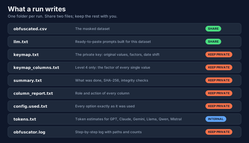
Each file has its own description in the Using the Program section (Output Files and Keymaps, LLM Prompts and Tokens).
6. Same input, same seed, same result
The random parts of a run (the date shift, the scaling factors and the hashed codes) come from a seed; the default is 42. Run the same input with the same options and the same seed and you get a byte-identical dataset; change the seed and the random parts change.
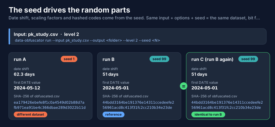
Sequential and padded identifier codes (1, 2, 3 and SUBJ001, SUBJ002) follow the order in which values first appear
in the file, so the seed does not change them. Use your own seed whenever privacy matters: the default 42 is public.
Where to go next
| Read | For |
|---|---|
| Workflows and Safety (next page) | the full workflows, which command to choose, what may be shared, what can be restored |
| Getting Started | installing and a first run, step by step |
| Using the Program | one page per command and per group of options, each with a tested example |